Getting started
To begin, a global view of how the code may be used is given here. Afterward, it is recommended to go through the two first examples provided below in order to get further step-by-step explanations.
General layout
The code make use of the possibilities provided by the object-oriented paradigm of python. In particular, the code tries to match physical components with objects (in the computer sense of the term) as much as possible.
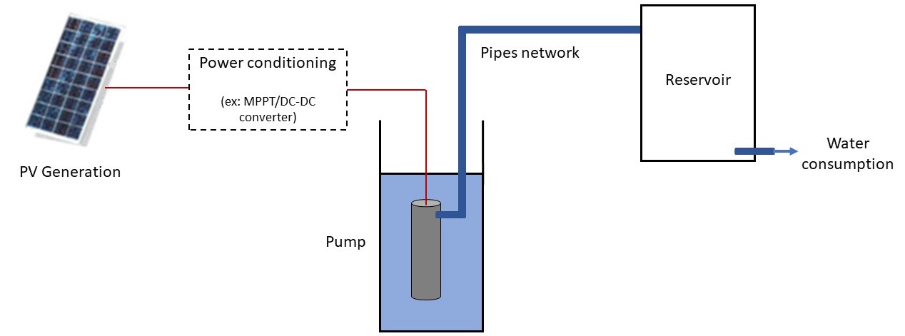
Therefore, modeling a PV pumping system requires to start by defining each object, i.e each component represented in below diagram.
Once all components have been declared in objects, they are gathered
in a parent object (an instance of class PVPumpSystem) where the type of
coupling between PV array and pump is declared.
Ultimately, the method run_model() launches the whole simulation.
It is also the step where the financial parameters can
be provided if a cost analysis is wanted.
Afterward, the results are contained in the object PVPumpSystem. At this point,
it is useful to have an IDE like Spyder or Pycharm to explore the values
internally contained. Otherwise, most of the results are actually stored in
the attributes flow, efficiency, water_stored, npv, llp.
The examples below, in particular the jupyter notebook ones, provide further details on each step of a standard simulation.
Examples
Three examples of how the software can be used are in the folder
docs/examples.
The examples are provided under two forms, as Jupyter Notebook files or as
Python files.
Jupyter Notebook
Following examples can be run locally with Jupyter Notebook, or by clicking on the corresponding icon in the upper right-hand corner of nbviewer pages, or by accessing through the binder build.
Simulation
The first two examples focus on simulation. These examples are important to understand because the modeling tools used here are the core of the software. These tools can be used later to get programs that fit a more particular use (for ex.: sizing process, parametric study, etc). For a given system, the examples show how to obtain the values of interest for the user (output flow rates, total water pumped in a year, loss of load probability (llp), net present value (npv), efficiencies and others):
Once you went through these 2 examples, you are quite ready to dive into the code and adapt it to your needs.
Sizing
The third example shows how to use a sizing function written from the modeling tools presented in the two examples above. This function aims at optimizing the selection of the pump and the PV module, based on user requirements.
Python files
These examples are also available in the form of python files in order to
freely adapt the code to your wishes. Directly check out in docs/examples.